Vector projection

Previous - Angles

Next - Matrices

Why vector projection

A projection of a vector onto another vector has many applications.

Imagine for example a cart on a slope. Given a vector made from two points on the slope and the gravity vector, we can use the projection of the gravitational acceleration vector onto the slope vector to calculate the direction and magnitude of the acceleration of the cart in a simple game physics setup.

Or think of the situation where a character jumps along an irregular polygon wall. When the collision circle of the character collides with the wall, we can calculate the closest point to the wall by projecting the circle’s center onto the wall.

If we want more precise collision detection and response, we can do this as well using vector projection, though we’ll need to learn a bit more about lines and polygons before we can get into that.

But before we can project points onto lines or start colliding polygons, we first need to get a basic understanding of how a vector can be projected onto another vector.

Calculating the projection of a vector onto another vector

If we look at the picture below, we see \(\vec{a_1}\) which is the projection of the vector \(\vec{a}\) onto \(\vec{b}\). The goal is to calculate \(\vec{a_1}\) in terms of \(\vec{a}\) and \(\vec{b}\).

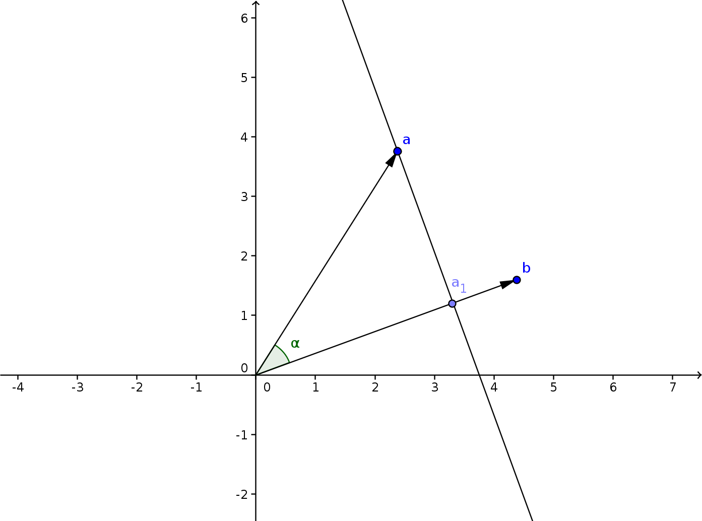
To make this task easier, or at least more intuitive, we are going to rotate this setup. Let’s arrange the vector \(\vec{b}\) so that it is parallel with the x-axis.

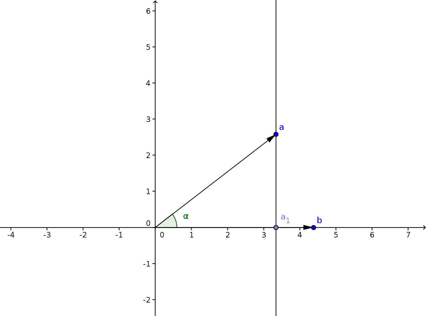
If we look at the vector \(\vec{a}\) now, we see that \(\vec{a_1}=\langle x, 0\rangle\) if \(\vec{a}=\langle x,y\rangle\). Now let’s scale our setup, so that \(\vec{a}\) is lying on the unit circle, a circle with as radius 1. In this case we see that \(x\) is equal to the cosine of \(\alpha\), which is the angle between \(\vec{a}\) and \(\vec{b}\).

\[x=cos(\alpha)\]

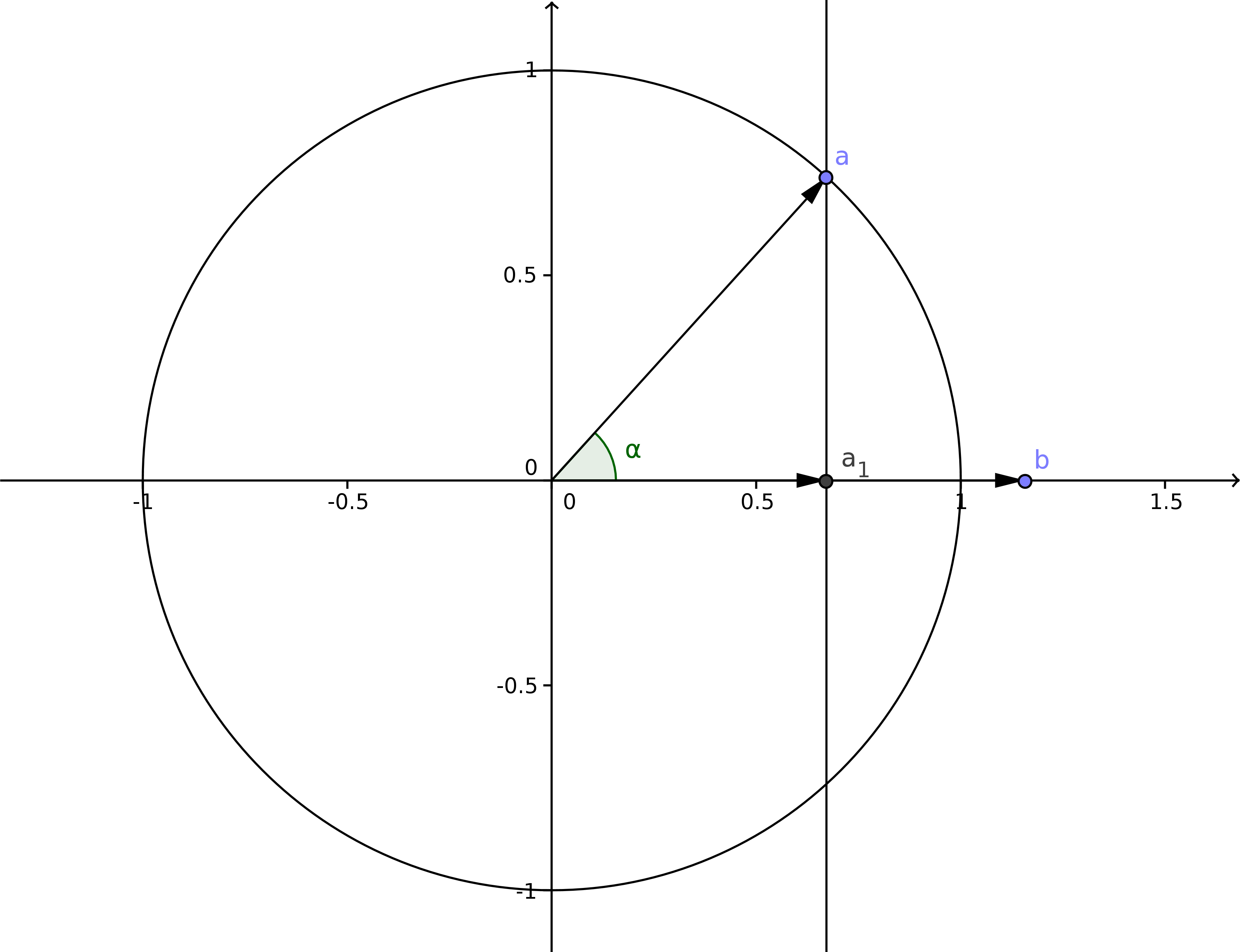
Of course in our second rotated but unscaled scenario, the vector \(\vec{a}\) doesn’t necessarily have a length equal to 1. Both \(\vec{a}\) and \(\vec{a_1}\) are scaled by the length of \(\vec{a}\). This means that to go back to the second scenario, have to multiply by the length of \(\vec{a}\) to correct the scale.

\[x=\lvert\vec{a}\lvert cos(\alpha)\quad(1)\]

As we stated before, we don’t want the angle \(\alpha\) in our equation, as we want a solution with just the two vectors \(\vec{a}\) and \(\vec{b}\). We can use the dot product, since the cosine of an angle is equal to the dot product of the vectors that form the angle if the vectors are normalized

\[cos(\alpha)=\hat{a}.\hat{b}\]

A normalized vector is one whose length is 1, thus it is obtained by dividing a vector by its length. Doing this with vectors \(\vec{a}\) and \(\vec{b}\) gives

\[cos(\alpha)=\frac{\vec{a}.\vec{b}}{\lvert \vec{a}\lvert\lvert \vec{b}\lvert}\quad(2)\]

Substituting the cosine in (1) by (2) gives

\[x=\lvert \vec{a}\lvert\frac{\vec{a}.\vec{b}}{\lvert \vec{a}\lvert\lvert \vec{b}\lvert}\]

Or simplified, since we can ignore multiplying and dividing by the same factor \(\lvert \vec{a}\lvert\)

\[x=\frac{\vec{a}.\vec{b}}{\lvert \vec{b}\lvert}\]

Our projection of vector \(\vec{a}\) in scenario 2 is was the vector \(\vec{a_1}=\langle x,0\rangle\) or \(\vec{a_1}=x\langle 1,0\rangle\), substituting \(x\) gives

\[\vec{a_1}=\frac{\vec{a}.\vec{b}}{\lvert \vec{b}\lvert}\langle1, 0\rangle\]

We chose \(\vec{b}\) to be parallel with the x-axis to clearly see that \(x\) was equal to the scaled cosine. But in our original scenario \(\vec{b}\) is not parallel to the x-axis. the only difference with scenario one and two is that we rotated everything. This rotation kept the sizes of the vectors as well as the angle between them intact. The only difference that affects the outcome is that \(\vec{b}\) is rotated. As we can see, the projected point \(\vec{a_1}\) always lies somewhere along \(\vec{b}\). In scenario two, \(\vec{a_1}\) only lies along the x-axis because \(\vec{b}\) is parallel with it. The vector \(\langle 1,0\rangle\) is nothing more than the normalized vector \(\hat{b}\). Thus our projection of \(\vec{a}\) on \(\vec{b}\) in scenario one is

\[proj(\vec{a},\vec{b})=\frac{\vec{a}.\vec{b}}{\lvert \vec{b}\lvert}\hat{b}\]

Since \(\hat{b}\) is equal to \(\vec{b}\) divided by it’s length \(\lvert \vec{b}\lvert\) we can write

\[proj(\vec{a},\vec{b})=\frac{\vec{a}.\vec{b}}{ {\lvert \vec{b}\lvert}^2}\vec{b}\]

And since the length \(\lvert \vec{b}\lvert\) is the square root of the dot product of \(\vec{b}\) with itself or \(\lvert \vec{b}\lvert=\sqrt{\vec{b}.\vec{b}}\) we get

\[proj(\vec{a},\vec{b})=\frac{\vec{a}.\vec{b}}{\vec{b}.\vec{b}}\vec{b}\]

So the projection of \(\vec{a}\) on \(\vec{b}\) is the dot product of \(\vec{a}\) and \(\vec{b}\) divided by the dot product of \(\vec{b}\) with itself multiplied with \(\vec{b}\).

function project(x1, y1, x2, y2)
    return mul(dot(x1, y1, x2, y2) / dot(x2, y2, x2, y2), x2, y2)
end

Projecting a point on a line

Now that we can project a vector onto another vector, it is easy to do things like projecting a point onto a line.

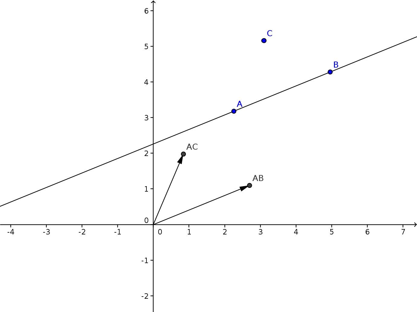
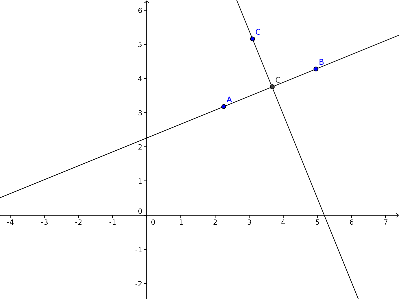
If we have a line AB defined by two points A and B on the line, and C the point we want to project, we build the vector \(\vec{AC}\), and project it onto the vector \(\vec{AB}\). From the resulting vector, \(\vec{AC'}\) we can then make the projected point C’ by adding A again.

Basically what happens is that first we translate everything so that A becomes the origin.

Then we project AC onto AB.

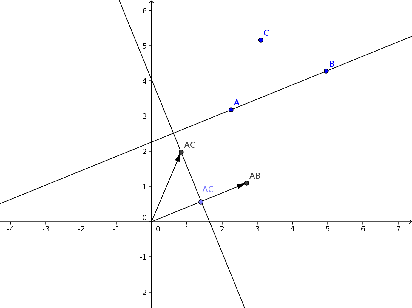
And finally we translate everything back where it was.

function projectPoint(px, py, x1, y1, x2, y2)
    return add(x1, y1, project(px-x1, py-y1, x2-x1, y2-y1))
end

Distance of a point to a line

We can now calculate the distance from a point to a line, as the projected point is the point on the line which lies closest to our point.

function distancePointLine(px, py, x1, y1, x2, y2)
    return distance(px, py, projectPoint(px, py, x1, y1, x2, y2))
end

Distance of a circle to a line

Similarly we can calculate the distance from a circle to a line. We just measure the distance between the circle center and the line, and subtract the radius.

function distanceCircleLine(cx, cy, radius, x1, y1, x2, y2)
    return distancePointLine(cx, cy, x1, y1, x2, y2) - radius
end

While you might be tempted to use this for collision detection, by checking whether the distance is negative, don’t forget we’re using a square root in our distance calculation, which we don’t need. A more optimal way is using the squared distance, and looking whether that is smaller than the square of the radius.

function collidesCircleLine(cx, cy, radius, x1, y1, x2, y2)
    local x, y = projectPoint(cx, cy, x1, y1, x2, y2)
    return distance2(x, y, cx, cy) < radius * radius
end

Remember, only use distances when you actually need the distance, for comparing distances, use squared distances instead.

Previous - Angles

Next - Matrices